Tutorial: Distinguishing attributes using ConceptNet
In a previous post, we mentioned the good results that systems built using ConceptNet got at SemEval this year. One of those systems was our own entry to the “Capturing Discriminative Attributes” task, about determining differences in meanings between words.
The system we submitted got second place, by combining information from ConceptNet, WordNet, Wikipedia, and Google Books. That system has some messy dependencies and fiddly details, so in this tutorial, we’re going to build a much simpler version of the system that also performs well.
Distinguishing attributes the simple way¶ 
Our poster, a prettier version of our SemEval paper, mainly presents the full version of the system, the one that uses five different methods of distinguishing attributes and combines them all in an SVM classifier. But here, I particularly want you to take note of the “ConceptNet is all you need” section, describing a simpler version we discovered while evaluating what made the full system work.
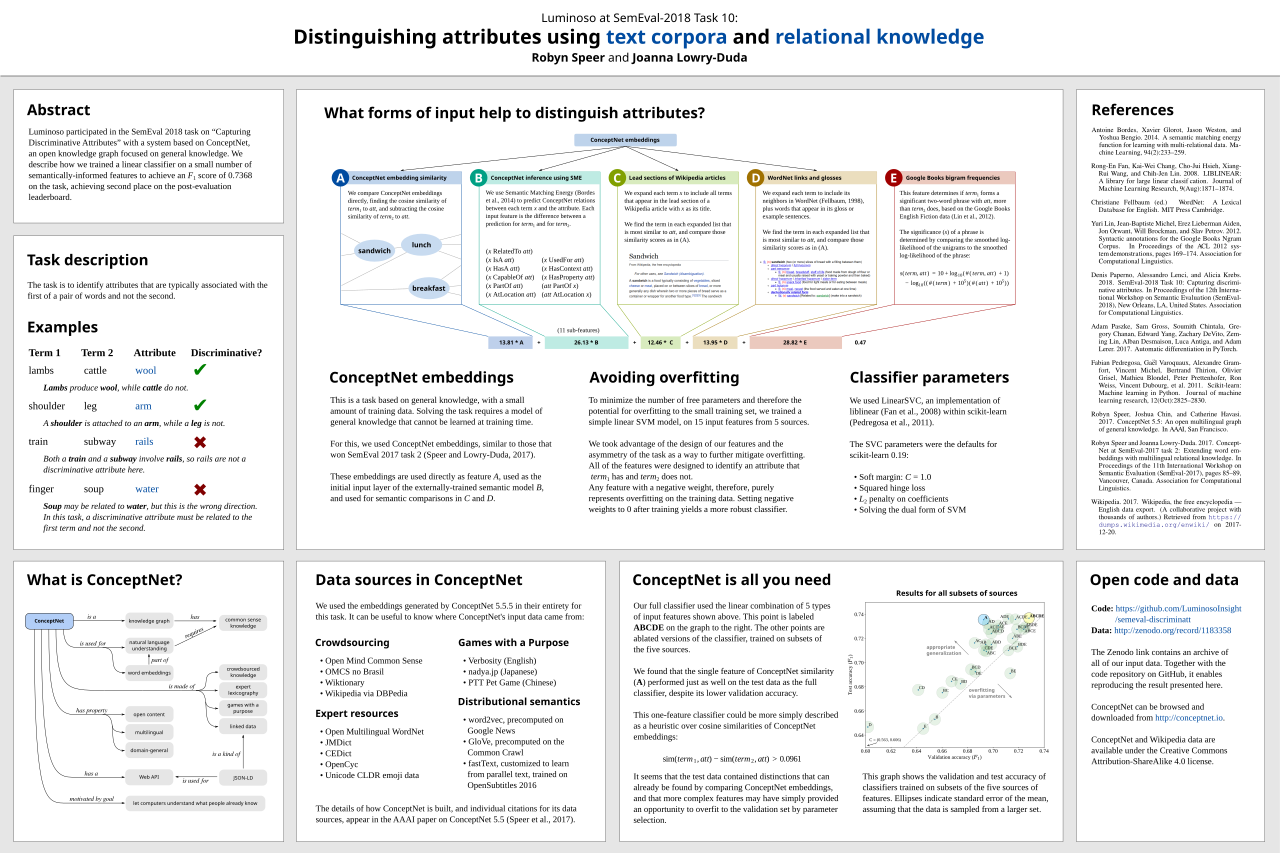
It seems that, instead of using five kinds of features, we may have been able to do just as well using just the pre-trained embeddings we call ConceptNet Numberbatch. So we’ll build that system here, using the ConceptNet Numberbatch data and a small amount of code, with only common dependencies (pandas and sklearn).
from sklearn.metrics import f1_score
import numpy as np
import pandas as pd
I want you to be able to reproduce this result, so I’ve put the SemEval data files, along with the exact version of ConceptNet Numberbatch we were using, in a zip file on my favorite scientific data hosting service, Zenodo.
These shell commands should serve the purpose of downloading and extracting that data, if the wget and unzip commands are available on your system.
!wget https://zenodo.org/record/1289942/files/conceptnet-distinguishing-attributes-data.zip
!unzip conceptnet-distinguishing-attributes-data.zip
In our actual solution, we imported some utilities from the ConceptNet5 codebase. In this simplified version, we’ll re-define the utilities that we need.
def text_to_uri(text):
    """
    An extremely cut-down version of ConceptNet's `standardized_concept_uri`.
    Converts a term such as "apple" into its ConceptNet URI, "/c/en/apple".

    Only works for single English words, with no punctuation besides hyphens.
    """
    return '/c/en/' + text.lower().replace('-', '_')

def normalize_vec(vec):
    """
    Normalize a vector to a unit vector, so that dot products are cosine
    similarities.

    If it's the zero vector, leave it as is, so all its cosine similarities
    will be zero.
    """
    norm = vec.dot(vec) ** 0.5
    if norm == 0:
        return vec
    return vec / norm
We would need a lot more support from the ConceptNet code if we wanted to apply ConceptNet’s strategy for out-of-vocabulary words. Fortunately, the words in this task are quite common. Our out-of-vocabulary strategy can be to return the zero vector.
class AttributeHeuristic:
    def __init__(self, hdf5_filename):
        """
        Load a word embedding matrix that is the 'mat' member of an HDF5 file,
        with UTF-8 labels for its rows.

        (This is the format that ConceptNet Numberbatch word embeddings use.)
        """
        self.embeddings = pd.read_hdf(hdf5_filename, 'mat', encoding='utf-8')
        self.cache = {}

    def get_vector(self, term):
        """
        Look up the vector for a term, returning it normalized to a unit vector.
        If the term is out-of-vocabulary, return a zero vector.

        Because many terms appear repeatedly in the data, cache the result.
        """
        uri = text_to_uri(term)
        if uri in self.cache:
            return self.cache[uri]
        else:
            try:
                vec = normalize_vec(self.embeddings.loc[uri])
            except KeyError:
                vec = pd.Series(index=self.embeddings.columns).fillna(0)
            self.cache[uri] = vec
            return vec

    def get_similarity(self, term1, term2):
        """
        Get the cosine similarity between the embeddings of two terms.
        """
        return self.get_vector(term1).dot(self.get_vector(term2))

    def compare_attributes(self, term1, term2, attribute):
        """
        Our heuristic for whether an attribute applies more to term1 than
        to term2: find the cosine similarity of each term with the
        attribute, and take the difference of the square roots of those
        similarities.
        """
        match1 = max(0, self.get_similarity(term1, attribute)) ** 0.5
        match2 = max(0, self.get_similarity(term2, attribute)) ** 0.5
        return match1 - match2

    def classify(self, term1, term2, attribute, threshold):
        """
        Convert the attribute heuristic into a yes-or-no decision, by testing
        whether the difference is larger than a given threshold.
        """
        return self.compare_attributes(term1, term2, attribute) > threshold

    def evaluate(self, semeval_filename, threshold):
        """
        Evaluate the heuristic on a file containing instances of this form:

            banjo,harmonica,stations,0
            mushroom,onions,stem,1

        Return the macro-averaged F1 score. (As in the task, we use macro-
        averaged F1 instead of raw accuracy, to avoid being misled by
        imbalanced classes.)
        """
        our_answers = []
        real_answers = []
        for line in open(semeval_filename, encoding='utf-8'):
            term1, term2, attribute, strval = line.rstrip().split(',')
            discriminative = bool(int(strval))
            real_answers.append(discriminative)
            our_answers.append(self.classify(term1, term2, attribute, threshold))

        return f1_score(real_answers, our_answers, average='macro')
When we ran this solution, our latest set of word embeddings calculated from ConceptNet was ‘numberbatch-20180108-biased’. This name indicates that it was built on January 8, 2018, and acknowledges that we haven’t run it through the de-biasing process, which we consider important when deploying a machine learning system.
Here, we didn’t want to complicate things by adding the de-biasing step. But keep in mind that this heuristic would probably have some unfortunate trends if it were asked to distinguish attributes of people’s name, gender, or ethnicity.
heuristic = AttributeHeuristic('numberbatch-20180108-biased.h5')
The classifier has one parameter that can vary, which is the “threshold”: the minimum difference between cosine similarities that will count as a discriminative attribute. When we ran the training code for our full SemEval entry on this one feature, we got a classifier that’s equivalent to a threshold of 0.096. Let’s simplify that by rounding it off to 0.1.
heuristic.evaluate('discriminatt-train.txt', threshold=0.1)
When we were creating this code, we didn’t have access to the test set — this is pretty much the point of SemEval. We could compare results on the validation set, which is how we decided to use a combination of five features, where the feature you see here is only one of them. It’s also how we found that taking the square root of the cosine similarities was helpful.
When we’re just revisiting a simplified version of the classifier, there isn’t much that we need to do with the validation set, but let’s take a look at how it does anyway.
heuristic.evaluate('discriminatt-validation.txt', threshold=0.1)
But what’s really interesting about this simple heuristic is how it performs on the previously held-out test set.
heuristic.evaluate('discriminatt-test.txt', threshold=0.1)
It’s pretty remarkable to see a test accuracy that’s so much higher than the training accuracy! It should actually make you suspicious that this classifier is somehow tuned to the test data.
But that’s why it’s nice to have a result we can compare to that followed the SemEval process. Our actual SemEval entry got the same accuracy, 73.6%, and showed that we could attain that number without having any access to the test data.
Many entries to this task performed better on the test data than on the validation data. It seems that the test set is cleaner overall than the validation set, which in turn is cleaner than the training set. Simple classifiers that generalize well had the chance to do much better on the test set. Classifiers which had the ability to focus too much on the specific details of the training set, some of which are erroneous, performed worse.
But you could still question whether the simplified system that we came up with after the fact can actually be compared to the system we submitted, which will leads me on a digression about “lucky systems” at the end of this post.
Examples¶ 
Let’s see how this heuristic does on some examples of these “discriminative attribute” questions.
When we look at heuristic.compare_attributes(a, b, c), we’re asking if a is more associated with c than b is. The heuristic returns a number. By our evaluation above, we consider the attribute to be discriminative if the number is 0.1 or greater.
Let’s start with an easy one: Most windows are made of glass, and most doors aren’t.
heuristic.compare_attributes('window', 'door', 'glass')
From the examples in the code above: mushrooms have stems, while onions don’t.
heuristic.compare_attributes('mushroom', 'onions', 'stem')
This one comes straight from the task description: cappuccino contains milk, while americano doesn’t. Unfortunately, our heuristic is not confident about the distinction, and returns a value less than 0.1. It would fail this example in the evaluation.
heuristic.compare_attributes('cappuccino', 'americano', 'milk')
An example of a non-discriminative attribute: trains and subways both involve rails. Our heuristic barely gets this right, but only due to lack of confidence.
heuristic.compare_attributes('train', 'subway', 'rails')
This was not required for the task, but the heuristic can also tell us when an attribute is discriminative in the opposite direction. Water is much more associated with soup than it is with fingers. It is a discriminative attribute that distinguishes soup from finger, not finger from soup. The heuristic gives us back a negative number indicating this.
heuristic.compare_attributes('finger', 'soup', 'water')
Lucky systems¶ 
As a kid, I used to hold marble racing tournaments in my room, rolling marbles simultaneously down plastic towers of tracks and funnels. I went so far as to set up a bracket of 64 marbles to find the fastest marble. I kind of thought that running marble tournaments was peculiar to me and my childhood, but now I’ve found out that marble racing videos on YouTube are a big thing! Some of them even have overlays as if they’re major sporting events.
In the end, there’s nothing special about the fastest marble compared to most other marbles. It’s just lucky. If one ran the tournament again, the marble champion might lose in the first round. But the one thing you could conclude about the fastest marble is that it was no worse than the other marbles. A bad marble (say, a misshapen one, or a plastic bead) would never luck out enough to win.
In our paper, we tested 30 alternate versions of the classifier, including the one that was roughly equivalent to this very simple system. We were impressed by the fact that it performed as well as our real entry. And this could be because of the inherent power of ConceptNet Numberbatch, or it could be because it’s the lucky marble.
I tried it with other thresholds besides 0.1, and some of the nearby reasonable threshold values only score 71% or 72%. But that still tells you that this interestingly simple system is doing the right thing and is capable of getting a very good result. It’s good enough to be the lucky marble, so it’s good enough for this tutorial.
Incidentally, the same argument about “lucky systems” applies to SemEval entries themselves. There are dozens of entries from different teams, and the top-scoring entry is going to be an entry that did the right thing and also got lucky.
In the post-SemEval discussion at ACL, someone proposed that all results should be Bayesian probability distributions, estimated by evaluating systems on various subsets of the test data, and instead of declaring a single winner or a tie, we should get probabilistic beliefs as results: “There is an 80% chance that entry A is the best solution to the task, an 18% chance that entry B is the best solution…”
I find this argument entirely reasonable, and probably unlikely to catch on in a world where we haven’t even managed to replace the use of p-values.
Comments
Comments powered by Disqus